RStudio 0.94.92 visited

I just updated my RStudio version to the latest, v.0.94.92 (will this asymptotically approach 1, or actually get to 1?). It was nice to see the number of improvements the development team has implemented, based I’m sure on community feedback. The team has, in my experience, been extraordinarily responsive to user feedback, and I’m sure this played a large part in the development path taken by the team. 

First and foremost, I was happy to see most of my wants met in this version:

• There now is a keyboard shortcut for <- that is easy and intuitive (Alt+_/Option+_)
• The File window now allows sorting by modification date  in addition to name, which was becoming an issue for one of my projects
• Plots can be saved as BMP, TIFF, JPEG and Postscript in addition to PNG and PDF
• Bracket completion and matching, very much similar to the R Mac GUI, and actually better than Emacs/ESS, specially when deleting.
• An easy shortcut to repeat blocks of text or transpose two lines of text (though this appears mistakenly overloaded with another shortcut on Windows/Linux)
• Keyboard shortcuts are reasonably consistent with OS-specific shortcuts, though the Ctrl key is used in Mac more than generally seen in the OS. It is however convenient for those of us migrating from Emacs/ESS, who use the Ctrl key often. 

My wishlist for RStudio is pretty much fulfilled with respect to R development. However, a few improvements need to be made in the TeX/Sweave interface to allow for autocompletion, templates, and fuller functionality in line with Emacs/Auctex and Texmate. Currently writing LaTeX and Sweave feels like writing in Wordpad, albeit with R-specific word completion and R functionality. This can be a bit more polished. Of course TeX and Sweave are still used by a minority of R users, so the fact that this functionality hasn’t developed is no surprise. 

All in all, the current version of RStudio feels like a very usable IDE for R, and certain features and similarities make migrating from Emacs pretty easy (provided you don’t miss Emacs’ overall power and flexibility too much)

A ggplot trick to plot different plot types in facets

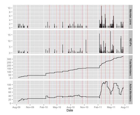
At the DC useR meetup last week, Marck Vaisman (@wahalulu) showed me a neat trick he’d learned to allow different facets in a faceted ggplot graph to have different plot types. The basis for this trick is this blog post in the Learn-R blog. Marck was trying to plot different statistics on our Meetup group’s membership on a faceted plot. Some of the variables were amenable to a step plot while others were more amenable to plotting using vertical lines.

The interesting trick in this example is to use the subset command within each geom to only layer one facet at a time. The source code is given below:

meetup <- read.csv('MeetupDates.csv', as.is=T)
names(meetup) <- 'Dates'
meetup$Dates <- as.Date(meetup$Dates,format='%m/%d/%y')
files  <- dir(pattern='DC_useR')
bl <- list()
for(f in files){
  bl[[f]] <- read.csv(f, as.is=T)
  bl[[f]]$Date <- as.Date(bl[[f]]$Date,format='%m/%d/%y')
}
dat <- Reduce(function(x,y) merge(x,y), bl) # Merge the data frames by Date
dat2 <- melt(dat,id=1)

# Here comes the trick !!
f1 <- ggplot(dat2, aes(x=Date,y=value,ymin=0,ymax=value))+facet_grid(variable~., scales='free')
f2 <- f1+geom_step(subset=.(variable=='Total.Members'))
f3 <- f2+geom_step(subset=.(variable=='Active.Members'))
f4 <- f3+geom_linerange(subset=.(variable=='Member.Joins'))
f5 <- f4+geom_linerange(subset=.(variable=='RSVPs'))
f5+geom_vline(xintercept=meetup$Dates, color='red',alpha=.3)+ylab('')

This produces the following plot:

A faceted ggplot object with different plot types

A word of warning about grep, which and the like

I’ve often selected columns or rows of a data frame using grep or which, based on some property. That is inherently sound, but the trouble comes when you wish to remove rows or columns based on that grep or which call, e.g.,

dat <- dat[,-grep('\\.1', names(dat))]

which would remove columns with a .1 in the name. This is fine the first time around, but if you forget and re-run the code, grep('\\.1',names(dat)) gives a vector of length 0, and hence dat becomes a data.frame with 0 columns. The function which also has similar pitfalls, as demonstrated in a recent R-help posting by David Winsemius. I find a more reliable method is to do

dat <- dat[,setdiff(1:ncol(dat),grep('\\.1',names(dat)))]

which will always give the right number of columns. Other suggestions for getting around this issue are welcomed in the comments.

SAS, R and categorical variables

One of the disappointing problems in SAS (as I need PROC MIXED for some analysis) is to recode categorical variables to have a particular reference category. In R, my usual tool, this is rather easy both to set and to modify using the  relevel command available in base R (in the stats package). My understanding is that this is actually easy in SAS for GLM, PHREG and some others, but not in PROC MIXED. (Once again I face my pet peeve about the inconsistencies within a leading commercial product and market “leader” like SAS). The easiest way to deal with this, I believe, is to actually create the dummy variables by hand using ifelse statements and use them in the model rather than the categorical variables themselves. If most of the covariates are not categorical, this isn’t too burdensome.

I’m sure some SAS guru will comment on the elegant or “right” solution to this problem.